ABL Profiling Made Easier with OpenEdge Profiler and ProPeek

What Is a .prof File and Why Is It Useful?

Profiling is the practice of recording the runtime behaviour of your code. The ABL Virtual Machine, or AVM, provides a built-in profiler that tracks which modules ran, how many times each line was executed, how long each call took and which modules called each other. This data is written to a .prof file.

Why does this matter? Because performance problems are difficult to solve when you're working on assumptions. A procedure might seem slow, but is the real issue of a database query, a loop that is running too many times, or a call to another huge module? Without profiling data, it's easy to spend hours adding MESSAGE statements and making changes that don't actually improve anything.

A profiler removes the guesswork. Instead of trying to figure out where the time is being spent, you can see exactly what is happening. The .prof file contains the information you need to identify slow parts of your program and understand how different parts of the code interact. The challenge is making sense of that data - which is where tools like ProPeek can help.

How to Generate a Proper .prof File

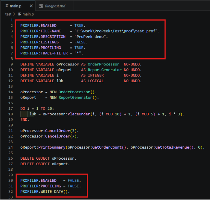
Generating a .prof file is straightforward, but the order of operations matters. The AVM has specific requirements for how you configure the PROFILER handle. Here is the correct sequence:

Step 1: Enable the profiler  

PROFILER:ENABLED = TRUE.

This must be set first. When you later set PROFILER:ENABLED = FALSE, the AVM automatically writes accumulated data to the output file and discards the module registry.

Note: if your ABL session exits while ENABLED is TRUE, profiling is automatically disabled to ensure data is written - so your profiling data is never silently lost.

Step 2: Set the output file path  

Set this immediately after ENABLED. The FILE-NAME attribute specifies where the .prof file will be written.

If you want to specify the folder, you can write a full path in FILE-NAME

PROFILER:FILE-NAME = "C:\path\myFirstProfile.prof".

Note: if you run multiple profiling sessions without changing FILE-NAME, each session overwrites the previous file.

Step 3: Configure optional attributes  

Before enabling profiling, you may want to set optional attributes. These are optional, but some are important enough that you should know when to use them:

• PROFILER:DESCRIPTION = “”: The description appears in the file header. It costs nothing to set, and when you're comparing two .prof files side by side, a clear description is what tells them apart.
• PROFILER:DIRECTORY: Sets the directory where listing files are saved. If not specified, listing files are saved in the current directory, even when a full path is provided in PROFILER:FILE-NAME.
• PROFILER:LISTINGS = TRUE: Generates .dbg debug listing files alongside the .prof output. This is important: when your procedures use {include.i} files or preprocessor directives, the profiler needs listings to map back to the correct source lines (useful feature of ProPeek). Without it, you will see compiled line numbers instead of source line numbers.
• PROFILER:COVERAGE:Tracks which executable lines were hit during the session. Useful for test coverage analysis. Requires PROFILER:LISTINGS = TRUE for accurate line mapping.
• PROFILER:TRACE-FILTER: Lets you filter which modules are included in tracing output, which helps manage file size when TRACE-FILTER is enabled.

Note: There is one attribute that the official documentation says to avoid: PROFILER:STATISTICS. "Avoid setting the STATISTICS attribute, as it produces large amounts of data. Enable it only if instructed by Technical Support." 

You can find more attributes here.

Step 4: Enable line-level profiling  

PROFILER:PROFILING = TRUE.

This turns on line-level timing data collection. It must be set after the attributes above.

Step 5: Run your application  

RUN myProcedure.p.

The profiler runs passively in the background from here. There is no other instrumentation needed in your application code.

Step 6: Stop profiling

There are two common ways to stop or pause profiling:

Option A: Simple teardown

PROFILER:ENABLED = FALSE.
PROFILER:PROFILING = FALSE. 

Setting ENABLED = FALSE automatically writes data to the file and stops profiling. This is the simplest approach for one-off profiling runs.

Option B: Intermediate writes

If you want to capture partial results without stopping the profiler, use WRITE-DATA():

PROFILER:PROFILING = FALSE. 
IF PROFILER:WRITE-DATA() THEN 
    MESSAGE "Profiler data written successfully." VIEW-AS ALERT-BOX. 
ELSE 
    MESSAGE "Failed to write profiler data." VIEW-AS ALERT-BOX. 

The WRITE-DATA() method returns TRUE on success or FALSE on failure, so you can check the result in a conditional. You can then set PROFILER:PROFILING = TRUE again to resume profiling.

Example of a simple profiling setup

To generate a useful .prof file, it is important to understand what information you actually need and use only the necessary attributes.

For example, if you don't need a detailed flame graph showing how many times the same method was called, you can set PROFILER:TRACE-FILTER = "" or simply not use it at all. This small change can reduce the size of the .prof file several times over, which is especially useful when working with very large profiling files.

What Does a Generated .prof File Contain?

The structure of the .prof file follows the Progress AVM Profiler Output Format, which defines the sections, fields and version differences described below.

The .prof file has several versions:

• Version 1: Initial implementation.
• ‍Version 2 – Same as Version 1, except it indicates that PROFILER:STATISTICS was enabled and so this output has 4 additional Statistics sections which follow the Code Coverage section.
• ‍Version 3: Same as Version 1, except it has a new Call-tree section, which follows the Code Coverage section and it has three minor changes to existing sections (detailed below).
• ‍Version 4: Same as Version 3, except it indicates that PROFILER:STATISTICS was enabled and so this output has 4 additional Statistics sections which follow the Code Coverage section.

Depending on the version, a .prof file is a text file with up to eight sections, separated by dots.

Main Sections of a .prof File

Header  

The header captures the identity and context of the profiling session. These is only one line of data for this section.

Format:

IntegerVersion Date "Description" SystemTime ""

IntegerVersion: version number of the profiler output format (1, 2, 3, or 4).

‍Date: date the profiler was enabled, in MM/DD/YYYY format.

Description: value of PROFILER:DESCRIPTION.

SystemTime: shows the time when the .prof was recorded in HH:MM:SS format

"" - an unused quoted string. In Version 3+ files, a JSON-formatted metadata object is appended here containing the PROPATH setting, the total profiling session time, and the total statement count.

Module data  

This section lists every module that participated in the profiling session and assigns each a session-unique integer identifier used by all subsequent sections. 

Format:

IntegerModuleID "ModuleName" "DebugListingFile" IntegerCRCVal

IntegerModuleID: session-unique integer identifier for this module. All following data will be in terms of these identifiers.

ModuleName: name of the module. It looks roughly like the output of PROGRAM-NAME function in Progress.

DebugListingFile: will be nil if PROFILER:LISTINGS was False when the module was first registered and it will be nil if the module is not an external procedure name or class file name (since they are the only ones that have debug listing files generated for them).

IntegerCRCVal: RCODE-INFO:CRC value computed over all sources comprising the .r file; 0 for modules that are not main .p or .cls files.

In Version 3+ files, two additional fields are appended to each record:

LineNum: line number in the source where the entry point is defined; 0 for main .p or .cls files.

Signature: currently always an empty string.

Call-graph

This section records every directed call edge observed during the session, capturing the complete call topology: which module called which, from which source line, and how many times.

Format:

CallerID CallerLineno CalleeID CallCount

CallerID: module ID of the calling module; 0 identifies the Session itself.

CallerLineno: line number in the calling module where the call was made; because this is included, multiple call sites from the same caller to the same callee are captured as separate records.

CalleeID: module ID of the called module.

CallCount: number of times this specific (caller, line, callee) combination was executed.

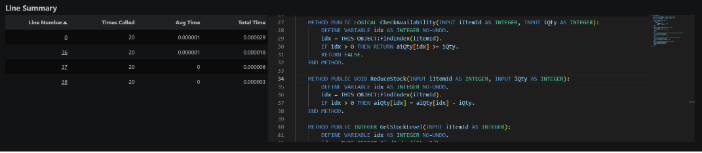
Line Summary  

This section provides per-line execution counts and timing for every source line that executed during the session.

Format:

ModuleID LineNo ExecCount ActualTime CumulativeTime

ModuleID: identifier of the module containing this line; 0 refers to the profiling session itself.

LineNo: source line number; 0 represents initialization and teardown overhead of the procedure, function, trigger, or method rather than any specific ABL statement.

ExecCount: number of times this line executed.

ActualTime: time in seconds spent directly executing this line only, excluding any time in called code.

CumulativeTime: time in seconds elapsed while this line ran, including all time spent in any code it invoked.

ExecCount of 1, an ActualTime of 0, and the CumulativeTime should reflect the total time for the profiling session. The CumulativeTime can be used to compute session percentages; e.g., what percentage of the session did Module X use.

Tracing Data  

Present only when PROFILER:TRACING or PROFILER:TRACE-FILTER is present, this section records one entry per individual statement execution - not per unique line - enabling full reconstruction of the execution timeline. A line that runs 1,000 times produces 1,000 records.

Format:

ModuleID LineNo ActualTime StartTime

ModuleID: identifier of the module containing this line.

LineNo: source line number of the executed statement.

ActualTime: time in seconds spent executing this single occurrence of the statement; microsecond precision.

StartTime: offset in seconds since the session's SystemTime (from the Header) recording when this execution began; microsecond precision.

Coverage Data  

Present only when PROFILER:LISTINGS = TRUE, this section enumerates the compiler-determined set of executable line numbers per module entry point.

Format:

ModuleID "EntryName" LineCount

ModuleID: identifies a top-level .p procedure or .cls class from the Module Data Section.

EntryName: name of the internal procedure, user-defined function, method, or trigger; nil if the record describes the executable lines of the main procedure body.

LineCount: number of executable lines in EntryName; exactly this many line-number records follow the header line.

Call-tree (Version 3+ only)  

This section provides a hierarchical view of the call chain with cumulative times per node, complementing the flat edge list of the Call-graph section by showing each module within its specific invocation context.

Format:

NodeID ParentNodeID ModuleID LineNum NumCalls CumulativeTime <n children NodeIds>

NodeID: Unique node in the call tree. Node 0 is the root node for the call-tree.

ParentNodeID: Node of the caller in the call tree.

ModuleID: The module id, from the Module section, for this node.

LineNum: The executable line number in the parent node (i.e., the line number in the caller where it called this node’s module).

NumCalls: Number of times this node was called by its parent node.

CumulativeTime: All time spent in this node and its children nodes.

<n children NodeIDs>:Variable number of children nodes which this node is calling.

Node 0 represents the Root node; it has a Parent NodeId, ModuleId, and LineNum of 0; NumCalls is 1; CumulativeTime is total time of the profiler run.

User Data Section  

This section contains free-text annotations that ABL application code writes into the profiler output by calling PROFILER:USER-DATA() at any point during the session. It is entirely application-defined and useful for marking meaningful phases, batch boundaries, or transaction identifiers within a long profiling run.

Format:

WriteTime "UserData"

WriteTime; offset in seconds since the session's SystemTime from the Header, recording exactly when the annotation was written.

UserData; the string val passed to the PROFILER:USER-DATA() method.

Here is what a fragment of the raw file actually looks like:

Special Line Numbers in Profiler Output

When looking at profiler output, either directly or through ProPeek, you may notice line numbers that do not represent real source lines.

Line 0

Line 0 represents overhead for initialising and tearing down a module, such as constructor and destructor cost. If a module shows meaningful time on line 0, it is spending that time on startup or cleanup rather than on a specific ABL statement.

Line -2

Line -2, present in Version 3+ .prof files, represents time spent on garbage collection within that module. If significant time appears on line -2, that module may be a source of garbage collection pressure, which can be useful when investigating memory behaviour.

Module identifiers, timestamps, call counts and line numbers are all available in the raw .prof file. However, reading this manually becomes impractical when a procedure calls dozens of modules across thousands of lines. This is exactly the gap ProPeek is designed to fill.

How ProPeek Visualises the .prof File

What is ProPeek?

ProPeek is a VS Code extension created by Baltic Amadeus. It opens .prof files and renders them as interactive visualisations. Instead of reading raw timing numbers, developers can explore graphs, trees and comparison views that make profiling data easier to understand.

ProPeek is useful for several scenarios:

• Diagnosing slow procedures;
• Understanding call chains;
• Comparing performance before and after a change;
• Spotting unexpected dependencies;
• Getting familiar with unfamiliar code.

This aligns with the purpose of the PROFILER handle: to locate bottlenecks and navigate the call tree to identify potential performance issues. ProPeek makes that navigation more visual and intuitive.

How to Open a .prof File with ProPeek

If you already have the ProPeek extension installed in VS Code, you can open a .prof file in just a few steps:

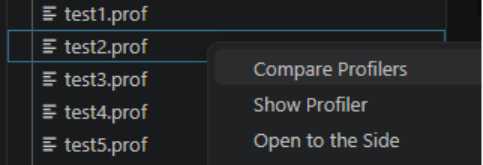
1. Right-click the .prof file in the Explorer.
2. Click “Show Profiler”.

This will open a structured visualization of the profiling data in ProPeek.

Module Details

The Module Details tab is made of 3 parts:

Module list

This section shows the list of modules and it's information.

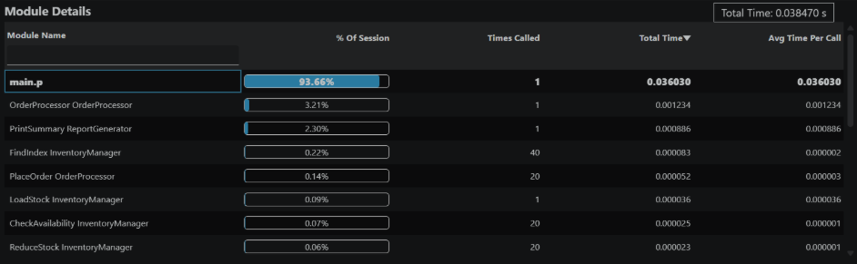
If you click on one of the modules, the information in the sections below will change to show the selected module statistics.

Note: If you generated .prof file with PROFILER:LISTINGS = TRUE, you can double-click on module name and the dbg_ code will open.

Calling Modules & Called Modules  

The relationship sections show the call graph from the perspective of the selected module:

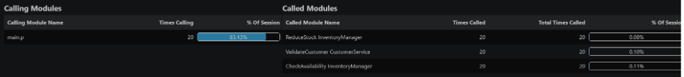
This section has 2 parts:

• Calling Modules: shows which modules called the selected module in the Module Details view. This helps you understand which call paths feed data into this module, and whether certain callers are responsible for most of the invocations.
• ‍Called Modules: shows which modules were called by the selected module in the Module Details view. This reveals whether this module is a lightweight coordinator (calls many other modules) or does most of its work in-house. If a module has high cumulative time but low actual time, it's a sign that it's called modules are the bottleneck.

Line Summary & Code Viewer  

The Line Summary section displays per-line execution statistics for every line of code executed in the selected module. It also shows the source code using Monaco Editor, the same editor used by VS Code.

Note: This feature works with profiler listing files generated using PROFILER:LISTINGS = TRUE. It also works with real source files when the profiled application belongs to a workspace that contains generated xref files (for example, after building with the Riverside OpenEdge extension). In that case, ProPeek uses xref information to resolve actual module locations and line numbers, including modules referenced through include files.

This tab is useful, because it shows you exactly which modules are hot and who calls it, pinpointing the specific code to optimize.

Tree View

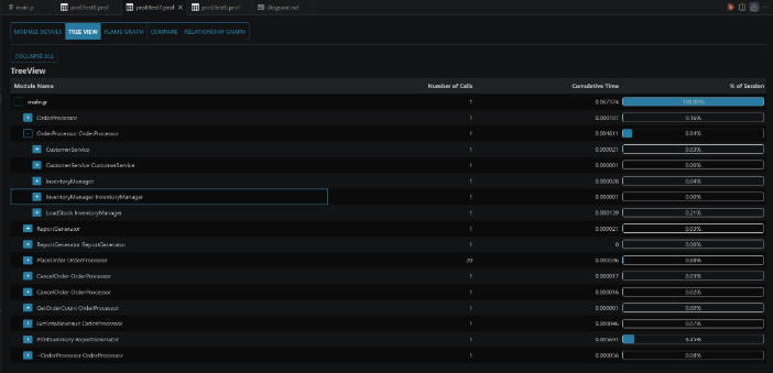
The Tree View displays the call-tree hierarchy as an expandable tree, showing the complete execution flow of your program from entry point to deepest call.

There are two useful features to know:

• Double-click a module: It opens the selected module in "Module Details" tab. This allows you to locate a module in a tree view and then analyze it in details.
• ‍Ctrl + click a module: It opens a dbg_ code of that module in VS Code, helping you identify what may cause memory or performance leaks.

This tab is useful, because it reveals the complete call chain from entry point to deepest function, helping you understand which execution path leads to your bottleneck.

Note: For Version 3+ profiler files, this view is built from the Call-tree section. For Version 1 profiler files, ProPeek reconstructs the hierarchy from the Tracing Data section using the same execution-trace information that is used to generate the Detailed Flame Graph.

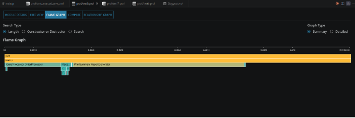
Flame Graph

There are some useful features to know:

• Flame Graph:A flame graph visualizes function and method calls, where each horizontal block represents a call and its width indicates the time spent executing it. The blocks are stacked vertically to show the call hierarchy, with taller stacks representing deeper levels of nested calls. By clicking on a block, you can expand it to the full width of the graph, making it easier to analyze the functions and methods called within that execution path.
• ‍Search Type
  
  • Length: Shows the default flame graph
  • ‍Constructor or Destructor: Highlights constructor and destructor calls while graying out all other blocks, making it easier to focus on object creation and destruction within the call hierarchy.
  • ‍Search: Allows you to search for a module by name, displays the number of matching nodes, and highlights the corresponding blocks in the graph. ‍
• ‍Graph Type
  
  • Summary: Flame graph shows the combined time of the same method if it was called several times in a row
  • ‍Detailed: Displays each invocation as a separate node and preserves exact timing information. In the Summary graph, child modules always begin at the left edge of their parent because only aggregated execution time is shown. In the Detailed graph, child modules appear at their actual execution position, which means a child call may start near the end of its parent if it was invoked late in the parent's lifetime.

Note: If there will be not enough information to generate a detailed flame graph, you will see this message:

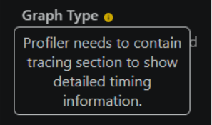
This tab is useful, because it visualizes time consumption as block width, instantly showing which functions are real bottlenecks without mental math.

Compare

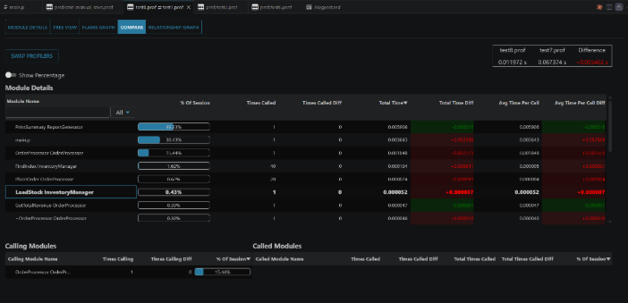
This tab lets you see a detailed comparison of two .prof files in one place.

You can open this tab in two ways:

1. Compare tab: If you already have a .prof file open in ProPeek, open the Compare tab. This will open a file explorer where you can select the second .prof file.
2. ‍Right-click: Right-click a .prof file and select “Compare Profilers”. This will open a file explorer so you can choose the second .prof file.
   

This tab is useful, because it lets you measure whether a code change actually improved performance or introduced unexpected regressions.

Relationship Graph

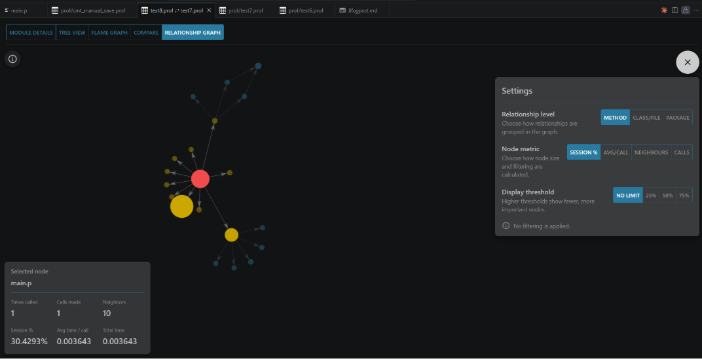
The Relationship Graph visualizes the call topology as a directed graph, showing the complete dependency structure of your application in a single, explorable visualization.

Graph Structure:

Nodes: each node represents a unique module (procedure, class, or method).

Edges: each directed edge represents a call from one module to another. An arrow points from caller to callee.

Node Size: larger nodes indicate modules with higher cumulative time (consuming more of the total profiling cost).

Edge Thickness: thicker edges indicate more calls between two modules (higher execution count for that call path).

Note: This graph maps directly to Section 3 (Call-graph) of the .prof file - the raw call-topology data. The relationship graph is its visual, explorable form.

This tab helps you:

• Spotting Unexpected Dependencies: in large ABL codebases, call chains are rarely obvious from reading the code. The Relationship Graph lets you see the dependency structure at a glance.
• ‍Finding Optimization Targets: central hub modules that everything depends on are candidates for optimization. Optimizing a heavily-called utility benefits the entire application.
• ‍Root Cause Analysis: if your flame graph shows a slow call chain, the relationship graph helps you trace it back to the entry point.

From Raw Profiling Data to Practical Performance Insights

The OpenEdge profiler is a powerful tool that is already available to ABL developers. It provides the data needed to understand and optimise application performance. However, the raw .prof file can be dense, difficult to interpret and easy to misread.

ProPeek helps close that gap.

By combining proper .prof generation with ProPeek’s interactive visualisations, profiling becomes a much more practical investigation process. Flame graphs show where time is being spent. The Relationship Graph reveals the application structure. Compare mode helps measure the impact of code changes.

If you have ever guessed at performance problems or spent hours optimising the wrong code, profiling can help bring the real issue into focus. With ProPeek, that process becomes more accessible for ABL developers.

Baltic Amadeus helps teams optimise and modernise Progress OpenEdge applications, identify performance bottlenecks and make complex ABL systems easier to maintain. Take a look at our Progress OpenEdge services.